Mandelbrot Set
Mandelbrot Set
The Mandelbrot set $M$ is defined by a uncountable set of complex quadratic polynomials,
\[f(z) = z^2 + z_0\], where the sample point $z_0$ is a complex parameter.
For each $z_0$, the sequence is obtained by iterating at each $z_0$, i.e.
The Mandelbrot set is defined such that the sequene is bounded and does not escape to infinity. This conditions constrained that the largeste complex number in the Mandelbrot set is $z_0 = -2$, i.e. the threshold for divergence, or equivalently,
\[|z_n| \leq 2, \quad\forall n \geq 0.\]Visualization with Density Plot
For density with $\text{Re}(z_0)$ on $x$-axis and $\text{Im}(z_0)$ on $y$-axis, such that
\[|z| = \sqrt{\text{Re}(z_0)^2 + \text{Im}(z_0)^2}\]The steps to visualization is as follows
- Define the 1D Mandelbrot Set function
Mand(z0, max_steps). - Define the 2D function
Mandelbrot(ext, Nxy, max_steps)to create a 2D array of points in the complex plane. - Show the plot with matplotlib.
Mand()
from numpy import *
def Mand(z0, max_steps):
    z = 0j      # 0j means 0+0i, a complex number
    for itr in range(max_steps):
        if abs(z) > 2:  # Stopping condition
            return itr  # Show count
        z = z*z + z0
    return max_steps
# Example
result = Mand(0.5 + 0.5j, 100)
print(result)
5
Mandelbrot()
- Initialize the 2D grid with
data. -
Nested
\[x = x_\text{min} + (x_\text{max}-x_\text{min}) \times \frac{i}{Nxy-1.00}\]forloop to map all points in complex plane.
For both $x$ and $y$, to ensure that each point is evenly spaced, each iterated steps is fractioned by the intervals, - Store the x, y value in each point of
data.
def Mandelbrot(ext, Nxy, max_steps):
    """
    ext[4] is an array of 4 values, [min_x, max_x, min_y, max_y]
    Nxy is an int for number of points in x or y of the matrix
    max_steps is inputed into Mand()
    """
    data = zeros((Nxy, Nxy))  # initialize 2D array with tuple (int,int)
    for i in range(Nxy):
        for j in range(Nxy):
            x = ext[0] + (ext[1]-ext[0]) * i/(Nxy-1.)   # 1. denotes a floating point number
            y = ext[2] + (ext[3]-ext[2]) * j/(Nxy-1.)
            data[i,j] = Mand(x+y*1j, max_steps)
    return data
# data is now a 2D array filled with integers.
# Example
data = Mandelbrot([-2,1,-1,1], 500, 1000)
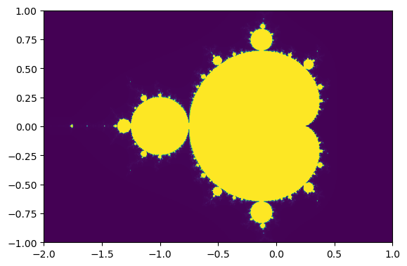
Density Plot
The module pylab in matplotlib is used to plot the 2D image, basically combining both numpy and matplotlib.pyplot in one namespace.
(Optional) To ensure the plot is displayed inline , we can use the magic command %matplotlib inline.
from pylab import *    # plotting library
%matplotlib inline

ext=[-2,1,-1,1]
# pylab's function for displaying 2D image
imshow(transpose(data), extent=ext)
show()
Time
To increase Nxy to 1000 would take a long time, we can use time to see how long it takes.
import time
t0 = time.time()
data = Mandelbrot([-2,1,-1,1], 1000, 1000)
t1 = time.time()
print('clock timed: ', t1-t0, 's.')
clock timed: 44.41298699378967 s.
Numba
The package numba is used to translate numpy into fast machine code to speed up the process. Numba’s JIT decorators, @jit, stands for “just-in-time” compilation for the python code to run at native machine code speed.
We will repeat the 2 functions above but with @njit, an alias for @jit(nopython=True), this time.
from numpy import * # because arrays are defined in numpy
from numba import njit  # This is the new line with numba

@njit   # this is an alias for @jit(nopython=True)
def Mand(z0, max_steps):
    z = 0j  # no need to specify type.
    # To initialize to complex number, just assign 0j==i*0
    for itr in range(max_steps):
        if abs(z)>2:
            return itr
        z = z*z + z0
    return max_steps

@njit
def Mandelbrot2(ext, Nxy, max_steps):
    """
    ext[4]    -- array of 4 values [min_x,max_x,min_y,max_y]
    Nxy       -- int number of points in x and y direction
    max_steps -- how many steps we will try at most before we conclude the point is in the set
    """
    data = zeros((Nxy,Nxy)) # initialize a 2D dynamic array
    for i in range(Nxy):
        for j in range(Nxy):
            x = ext[0] + (ext[1]-ext[0])*i/(Nxy-1.)
            y = ext[2] + (ext[3]-ext[2])*j/(Nxy-1.)
            # creating complex number of the fly
            data[i,j] = Mand(x + y*1j, max_steps)
    return data
# data now contains integers.
# MandelbrotSet has value 1000, and points not in the set have value <1000.
import time            # timeing
t0 = time.time()
data = Mandelbrot2(array([-2,1,-1,1]), 1000, 1000)
t1 = time.time()
print ('clock timed: ',t1-t0,'s')
clock timed: 4.229031085968018 s
It is around twice as fast using numba.
We can further speed up by using the following techniques:
- Pre-allocated arrays outside the functions to avoids dynamic memory allocation during the computation.
@njit(parallel=True): Numba (nopython) with parallelization.- Parallelization with prange for only the inner loop (j) to distributes work across multiple CPU cores for faster execution.
- Avoiding type checking: Numba eliminates Python’s runtime type-checking overhead.
from numpy import * # because arrays are defined in numpy
from numba import njit  # This is the new line with numba
from numba import prange

@njit   # this is an alias for @jit(nopython=True)
def Mand(z0, max_steps):
    z = 0j  # no need to specify type.
    # To initialize to complex number, just assign 0j==i*0
    for itr in range(max_steps):
        if abs(z)>2:
            return itr
        z = z*z + z0
    return max_steps

@njit(parallel=True)
def Mandelbrot3(data, ext, max_steps):
    """
    ext[4]    -- array of 4 values [min_x,max_x,min_y,max_y]
    Nxy       -- int number of points in x and y direction
    max_steps -- how many steps we will try at most before we conclude the point is in the set
    """
    Nx,Ny = shape(data) # 2D array should be already allocated we get its size
    for i in range(Nx):
        for j in prange(Ny):    # note that we used prange instead of range.
                                # this switches off parallelization of this loop, so that
                                # only the outside loop over i is parallelized.
            x = ext[0] + (ext[1]-ext[0])*i/(Nx-1.)
            y = ext[2] + (ext[3]-ext[2])*j/(Ny-1.)
            # creating complex number of the fly
            data[i,j] = Mand(x + y*1j, max_steps)
# data now contains integers.
# MandelbrotSet has value 1000, and points not in the set have value <1000.
import time            # timeing
data = zeros((1000,1000))
t0 = time.time()
Mandelbrot3(data, array([-2,1,-1,1]), 1000)
t1 = time.time()
print ('clock timed: ',t1-t0,'s')
clock timed: 2.2649178504943848 s
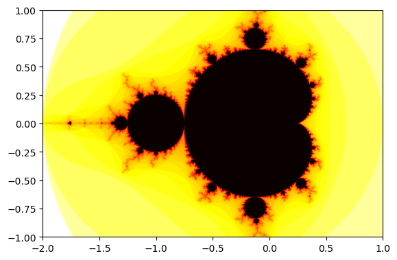
Density Logplot
We can use the the negative logarithm so that the Mandelbrot set has the smallest value. The logarithm enhances contrast by compressing large values (e.g., escape times) into a smaller range.
To use a different color map, use matplotlib.cm.
import matplotlib.cm as cm

# data.T is the transpose function
imshow(-log(data.T), extent=[-2,1,-1,1], cmap=cm.hot)
show()
Interactive Mandelbrot Set
- Get the New View Area: It retrieves the current visible bounds of the axes
(xstart, xend, ystart, yend). - Recompute Mandelbrot Data: It calls
Mandelbrot3()to recalculate the fractal data for the new visible area. - Update the Image:
Updates the image with the new fractal data
(-log(data.T)). Adjusts the image’s extent to match the visible area. - Redraw the Plot: It redraws the figure to display the updated fractal.
def ax_update(ax):  # actual plotting routine
    ax.set_autoscale_on(False) # Otherwise, infinite loop
    # Get the range for the new area
    xstart, ystart, xdelta, ydelta = ax.viewLim.bounds
    xend = xstart + xdelta
    yend = ystart + ydelta
    ext=array([xstart,xend,ystart,yend])
    Mandelbrot3(data, ext, 1000) # actually producing new fractal

    # Update the image object with our new data and extent
    im = ax.images[-1]  # take the latest object
    im.set_data(-log(data.T))   # update it with new data
    im.set_extent(ext)           # change the extent
    ax.figure.canvas.draw_idle() # finally redraw
To allow interactive window to show up from Jupyter Notebook in VScode, we have to change the matplotlib backend to qt and the interactive backend will become qtagg.
import matplotlib
%matplotlib qt
import matplotlib.pyplot as plt
print(matplotlib.get_backend())
qtagg
data = zeros((1000,1000))
ext=[-2,1,-1,1]
Mandelbrot3(data, array(ext), 1000)

fig,ax = plt.subplots(1,1)
ax.imshow(-log(data.T), extent=ext, aspect='equal',origin='lower',cmap=cm.hot)

ax.callbacks.connect('xlim_changed', ax_update)
ax.callbacks.connect('ylim_changed', ax_update)
plt.show()
In a separate file mandelbrot.py, you can run the script simply with python mandelbrot.py with terminal in the appropriate enviroment.